K Nearest Neighbors – Deep Dive

Much of Machine Learning involves finding and exploring patterns in data. ML algorithms will typically learn patterns from training data and apply what is learned on new data. One algorithm deviates slightly from this method, however; instead choosing to discover patterns as it encounters new data. K Nearest Neighbours (KNN for short) is an algorithm that can be applied to classification and regression problems. It’s probably one of the simplest algorithms in all of machine learning.

Basically, it works by assigning a value to a sample based on the values assigned to the K most similar samples already observed. Similarity among samples is evaluated by a ‘distance function’ which typically would vary according to the specific context of the problem you are trying to solve. The distance function accepts two samples and outputs a value indicating their similarity or closeness.

For classification problems, the labels of the K most similar samples are used in a majority voting scheme with the most occurring vote being assigned as the sample class. For regression problems, the outputs of the K most similar samples are averaged and the mean is assigned as the output for the new observed sample.

KNN is often referred to as a lazy learning algorithm. This is because as opposed to learning a model upfront on training data, KNNs learn relationships as new data is encountered. Essentially, a KNN algorithm will have access to some training data, but rather than computing a prediction model on the training data, it delays that process until when making predictions. For a new sample encountered, the algorithm computes the distance between that sample and all the training samples. The top K closest samples are employed in deciding what to assign our new sample. Seems straightforward right?

Here’s a visual that can aid in understanding: 

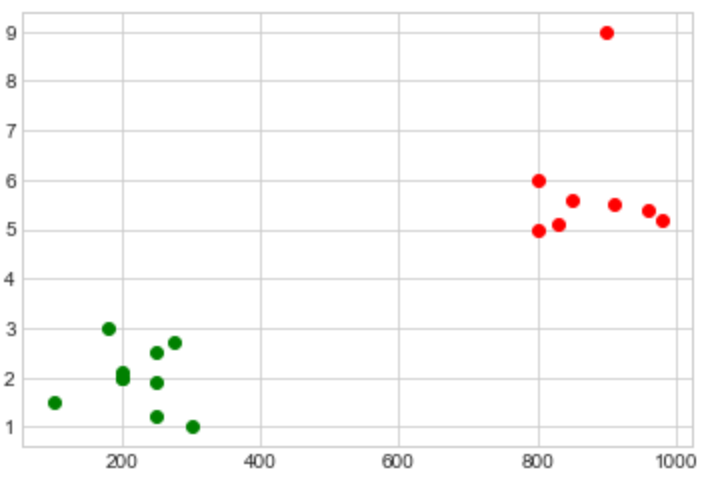
In the graph above, we have a clear separation of classes. Points to the left belong to the green class, and points to the right belong to the red class. Say we encountered a new point P with coordinates (250, 3.2). We don’t know which class to assign this new point, but because we know its features (coordinates in this case), we can place it on the graph and come up with a good prediction.

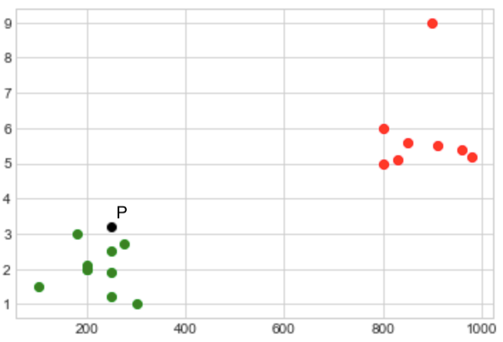
KNN evaluates the distance between Point P and the remaining points. If we set K as 5, chances are the closest 5 points will be green. Hence P is assigned the green class. The tricky part comes when trying to decide what value to use as K. Whatever that value may be, it can’t be too large or too small. Let’s see why. 

We already know that K is a parameter that determines the number of close occurring samples to use in prediction. What happens when K is too small? Well, for starters, we may not have enough quality votes to drive correct predictions. This is more likely to happen if we have a dataset that is skewed in a direction that isn’t fairly balanced. The K Nearest Neighbours will vote for the wrong answer because we have more examples of the wrong class. There are ways to mitigate this though, as we’ll explore later on. And when K is too large, the decision boundaries become less obvious and we run the risk of incorporating extraneous data in our predictions. Later on, we will run through techniques for choosing appropriate K values. 

What are some applications of KNN?

While KNNs can be applied to classification and regression problems, there are some problems for which they have gained popularity. KNNs for instance have been successfully applied to Recommender Systems. These systems are able to recommend similar items to a search query, and they exist in different forms:

• A movie website that recommends similar movies to the ones a user has watched
• A books website that recommends similar books to the ones user has already read.
• An e-commerce site that recommends similar products to the ones already on the user’s shopping cart. etc.

In fact, this kind of search is often called KNN Search ie “search items similar to this query”. The point is, if we can come up with a representation for a sample within a vector space, each feature would represent the magnitude of the vector along a dimension. Then we can apply KNN in searching for similar samples within that vector space.

The KNN algorithm

1. Store Training Data in an accessible location
2. Set an Initial value of K depending on the number of neighbors
3. For each sample in Training Data    
   i. Evaluate the distance between the query item and the current sample
   ii. Add a mapping of sample index and the distance to a collection
4. Sort the collection of sample indices and distances in increasing order of distance from smallest to largest
5. Select the first K entries from the collection
6. For a classification problem, choose the mode of the classes from the K samples
7. For a regression problem, choose the mean of the labels from the K samples

For a KNN search problem, you can imagine we would probably stop at step 5. We just want the K most similar items matching the query. 

More interesting though, is how we intend to define our distance Function. Whatever this function is, it will take into account the features of each sample. By features, I mean the specific characteristics of a sample that influence our prediction on that sample. Say we have a Movie Recommender System, we may choose to capture features like movie genre, rating, year of release. These features will be used to evaluate the distance between movie samples. There are a number of techniques that have been successfully applied to KNN distance problems. Most notable is Euclidean Distance. 

Euclidean Distance in Vector Spaces

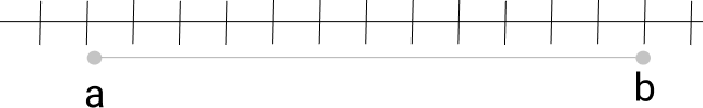
Mathematics tells us that the Euclidean distance between two points on a Vector Space is the straight line distance between them. For a one dimensional plane, the euclidean distance between points a and b is given as

   

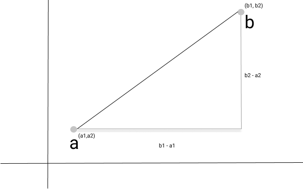
For a two dimensional plane, the euclidean distance is solved by the Pythagorean approach. 

   

The pythagorean approach still works for higher dimensions. In a three dimensional plane for instance, 

   

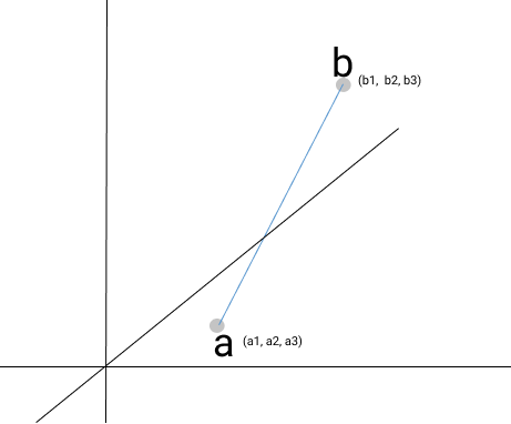
And so, we can generalise a formula for Euclidean distance:

   

If each feature corresponds to a dimension in our n-dimensional space, we can use the euclidean formula to evaluate the distance between two samples in that vector space. For two samples in our dataset, if they have similar features, they appear close to each other. 

But there’s a slight problem we need to address. We can run into scenarios where one particular feature might dominate our distance function. Say, for instance, we are inspecting space datasets which include samples from distant star systems. Each star system has two features: the size of the star (in million kilometers) and the number of revolving planets. If we wish to compute Euclidean distance for star systems, the size of the star is going to dominate our euclidean distance because the values are on a much larger scale than the number of revolving planets. This introduces a need for Feature Scaling. 

With Feature Scaling, we intend to transform the features into a range where they appear within the same scale while maintaining essential properties of the distribution. Normalization in statistics presents itself as a good technique for feature scaling. A technique where we compute the mean (u) and standard deviation (s) for the entire distribution, and for each sample, subtract the mean and divide by the standard deviation. 

   

Let’s see an example. 
If we have our star systems dataset with a few samples like this:

SN	planet_count	size (million km)
1	11	1,700,000
2	8	2,000,000
3	4	5,000
4	10	40,000,000

For the planet counts, the mean is 8.25 and the standard deviation is 2.680951323690902.

For the size column, the mean is 10,926,250 and the standard deviation is 16,802,963.0478526.

If we apply the normalization formula on each item, the result is what we have below. Both planet count and star size have been scaled to the same range and neither is likely to dominate the other. 

SN	planet_count	size (million km)
1	1.025755289064345	-0.5490847060723755
2	-0.09325048082403138	-0.5312307121071445
3	-1.5852581740085334	-0.6499597719759307
4	0.6527533657682196	1.7302751901554505

Wrapping Up

This note was the first in a series of notes that intend to dive into the K-Nearest Neighbour algorithm. We discussed the K-NN algorithm and its application. We also talked about Euclidean distance and how it relates to the K-NN algorithm. Finally, we touched on Normalisation as a means of standardizing datasets. In the next note, I will implement recommender systems using the concepts highlighted in this note. ciao.

Further Reading

• K Nearest_Neighbors Algorithm
• Euclidean Distance
• Normalization