The most basic form of machine learning you can do is a Simple Linear Regression. Remember in an earlier post, I mentioned that Supervised Learning is a form of machine learning in which we utilize training data to teach our algorithm to derive a function that can make predictions on new data. SLR is a kind of supervised learning where the function we seek to derive is a straight-line function.
From our understanding of straight-line graphs, we know they usually are of the form y = mx + b. Where m is the gradient of the line, b is the intercept on the y-axis when x is zero, x is the independent variable, and y is the dependent variable. In Machine learning parlance, we can also say x is the regressor and y is the regressand.
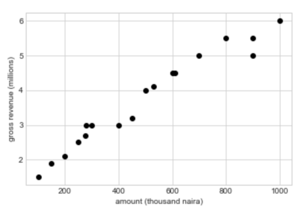
Let us imagine a problem. Say a company wishes to model a relationship between the amount spent on advertising expenses and the gross revenue realized in the time period (limited to one month). For this problem, the independent variable (x) is the amount spent on advertising, and the dependent variable (y) is the gross revenue made within the month. Of course, this is a fairly contrived example. In actuality, the gross revenue a company makes will depend on a lot more than just the advertising expenses. Assuming the company did well to gather data over the past 18 months in CSV format, below is a graph of our training data.
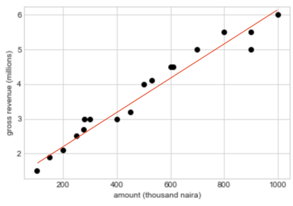
Somewhere in the 2-dimensional space, we hope to fit a hyperplane that will serve as our regression line and allow us to predict y values for x instances we do not have. A hyperplane is a subspace that is 1 dimension less than it’s surrounding space. In SLR, our vector space is 2-dimensional, comprising the amount spent on the x-axis, and the gross revenue on the y-axis. Our hyperplane is thus a straight line that best fits our data.
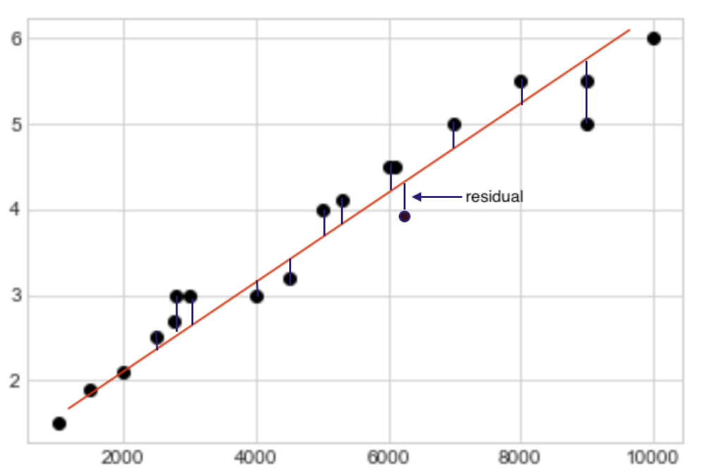
The question now is: how do we derive the regression line? First, we define a cost function that signifies the ‘wrongness’ of our model. This function is basically the sum of our squared residuals. For each training sample, the residual is the difference between the gross revenue predicted by our model and the actual gross revenue realized by the company.
The cost function is also called the residual sum of squares (RSS). We can write the formula for our cost function as:
![\[RSS = \sum_{i=1}^{N}({y_i-f(x_i)})^2\]](https://julianduru.com/wp-content/ql-cache/quicklatex.com-165e1af6b1ea6ec1f0718550d57af531_l3.png "Rendered by QuickLaTeX.com")
For all instances in training, we sum the square of the difference of y (observed actual value) and f(x) (value predicted for x). Surely, a higher value for our RSS indicates our model is very erroneous and will predict wrong values for x. A smaller value indicates the opposite. An appropriate model should minimize the cost function because our predictions will be very close to reality.
Now we have defined our RSS, let’s go back to our model. We know that: f(x) = mx + b. In the process of fitting our model on the training data, we intend to derive the parameters m and b that will minimize our RSS for all x. We can replace f(xi) in our RSS with mx + b. Hence our RSS is now,
![\[R = \sum_{i=1}^{N}({y_i-mx_i-b})^2\]](https://julianduru.com/wp-content/ql-cache/quicklatex.com-26138bcb9a861c96051a2addefaa1529_l3.png "Rendered by QuickLaTeX.com")
We can see that the RSS is a quadratic equation of some sort. And from our understanding of calculus, for a quadratic equation of the form y = ax2 + bx + c, at the minimum point, the derivative of y with respect to x equals 0. In this case, we take the partial derivative of R with respect to b and m. First, let’s evaluate with respect to b. We apply the chain rule in calculus, setting u as yi – mxi – b.
![\[\frac{\partial R}{\partial b} = \frac{\partial R}{\partial u} \times \frac{\partial u}{\partial b}\]](https://julianduru.com/wp-content/ql-cache/quicklatex.com-3869d9cc07367bf3df4457b61012a158_l3.png "Rendered by QuickLaTeX.com")
![\[\frac{\partial R}{\partial b} = \sum_{i=1}^{N}2(y_i-mx_i-b) \times -1\]](https://julianduru.com/wp-content/ql-cache/quicklatex.com-ab958ec82cac3e56eb30ba3cdad04db0_l3.png "Rendered by QuickLaTeX.com")
![\[\frac{\partial R}{\partial b}= \sum_{i=1}^{N}-2(y_i-mx_i-b)\]](https://julianduru.com/wp-content/ql-cache/quicklatex.com-bb020a94796b8a1c3294de9c5f68446a_l3.png "Rendered by QuickLaTeX.com")
At the point where the partial derivative equals 0, we have:
![\[0 = \sum_{i=1}^{N}-2(y_i-mx_i-b)\]](https://julianduru.com/wp-content/ql-cache/quicklatex.com-4e88045a03225a60c97ac8a5bdf5721a_l3.png "Rendered by QuickLaTeX.com")
Divide both sides by -2 and spread out the summation operator. We now have:
![\[0 = \sum_{i=1}^{N}y_i - \sum_{i=1}^{N}mx_i - \sum_{i=1}^{N}b\]](https://julianduru.com/wp-content/ql-cache/quicklatex.com-4a41f9f740ab2e500fca40bd71c9bffb_l3.png "Rendered by QuickLaTeX.com")
![\[0 = \sum_{i=1}^{N}y_i - \sum_{i=1}^{N}mx_i - bn\]](https://julianduru.com/wp-content/ql-cache/quicklatex.com-1c6e74b69e215403631f4d750eda3fd6_l3.png "Rendered by QuickLaTeX.com")
![\[b = \frac{\sum_{i=1}^{N}y_i - m\sum_{i=1}^{N}x_i}{n}\]](https://julianduru.com/wp-content/ql-cache/quicklatex.com-2fbd12b568ff3a4aa99fc1ae09825079_l3.png "Rendered by QuickLaTeX.com")
Through our understanding of statistics, we know that the mean of a bunch of numbers is the sum of those numbers divided by their count. We can insert the mean values for x and y in the equation, like this:
![\[b = \=y - m\=x\]](https://julianduru.com/wp-content/ql-cache/quicklatex.com-2bf5766aba2cc703dc9529dc64f922da_l3.png "Rendered by QuickLaTeX.com")
So we’ve been able to devise a formula for deriving one of our model’s parameter b. Given our training data, we can compute the mean for the x and y values, that is, the average amount spent on advertising every month and the average gross revenue made. But we are still missing the value m. To evaluate m, we take the partial derivative of R with respect to m. Again we apply the chain rule.
![\[\frac{\partial R}{\partial m} = \frac{\partial R}{\partial u} \times \frac{\partial u}{\partial m}\]](https://julianduru.com/wp-content/ql-cache/quicklatex.com-2c6469be6c34067ba5dde06da049049c_l3.png "Rendered by QuickLaTeX.com")
![\[\frac{\partial R}{\partial m} = \sum_{i=1}^{N}2(y_i-mx_i-b) \times -x_i\]](https://julianduru.com/wp-content/ql-cache/quicklatex.com-6b40baefbc8ee05208de922ffdd6c2d3_l3.png "Rendered by QuickLaTeX.com")
![\[\frac{\partial R}{\partial m} = \sum_{i=1}^{N}-2x_i(y_i-mx_i-b)\]](https://julianduru.com/wp-content/ql-cache/quicklatex.com-8218c82eaae0f6832f4b7302a4a8b4e5_l3.png "Rendered by QuickLaTeX.com")
At the point where the partial derivative equals 0, we have:
![\[0 = \sum_{i=1}^{N}x_i(y_i - mx_i - b)\]](https://julianduru.com/wp-content/ql-cache/quicklatex.com-e7c6980b896cda86edb9acffc019400b_l3.png "Rendered by QuickLaTeX.com")
![\[0 = \sum_{i=1}^{N}(x_iy_i - mx_i^2 - bx_i)\]](https://julianduru.com/wp-content/ql-cache/quicklatex.com-6a149768913853745a903fb46651a143_l3.png "Rendered by QuickLaTeX.com")
We already have a formula for b which we can insert in the equation.
![\[0 = \sum_{i=1}^{N}(x_iy_i - mx_i^2 - (\=y - m\=x)x_i)\]](https://julianduru.com/wp-content/ql-cache/quicklatex.com-af0299f9b8f57de5ebb32634137c3842_l3.png "Rendered by QuickLaTeX.com")
Now the equation is in terms of m, xi, and yi, we can simply make m the subject of the equation.
![\[0 = \sum_{i=1}^{N}(x_iy_i - mx_i^2 - x_i\=y + mx_i\=x)\]](https://julianduru.com/wp-content/ql-cache/quicklatex.com-a1b883b0d97942adbd7aa13c5d0df524_l3.png "Rendered by QuickLaTeX.com")
![\[0 = \sum_{i=1}^{N}(mx_i\=x - mx_i^2) + \sum_{i=1}^{N} (x_iy_i - x_i\=y)\]](https://julianduru.com/wp-content/ql-cache/quicklatex.com-9586fe89ca58ae261b0e101cfa9be0ae_l3.png "Rendered by QuickLaTeX.com")
![\[m = \frac{\sum_{i=1}^{N} (x_iy_i - x_i\=y)}{\sum_{i=1}^{N}(x_i^2 - x_i\=x)}\]](https://julianduru.com/wp-content/ql-cache/quicklatex.com-735424f2974f2539ea7cdbeb3bd0e5ae_l3.png "Rendered by QuickLaTeX.com")
Turns out, the above equation is also equal to the covariance of x and y divided by the variance of x. That is,
![\[m = \frac{cov(x, y)}{var(x)}\]](https://julianduru.com/wp-content/ql-cache/quicklatex.com-12e247a84a5689b7cbe4e73852f5fdcd_l3.png "Rendered by QuickLaTeX.com")
Let us quickly define some of these terms.
The covariance of two variables gives the degree of joint variability. That is, how the variables change together. If higher values of one variable coincide with higher values of the other variable and vice versa, then we have positive covariance. But if higher values of one variable coincide with lower values of the other variable, then we have a negative covariance. Hence, if cov(x, y) is positive, then higher values of x will also result in higher values of y. The hyperplane will trend upward from left to right.
Variance is a concept in statistics that allows us to evaluate the extent to which data items are spread from their mean. A higher variance indicates values are more spread out, while lower variance indicates values are more clustered.
Now we have the formulas for deriving the parameters of our hyperplane that will minimize our cost function. It’s time to write some code.
We have assembled our training data into a CSV File containing two columns. Below is a code snippet to help us extract the x and y values for our training set.
import numpy as np
import pandas as pd


def read_data(x_header, y_header):
    path = input('Enter path to CSV file: ')
    frame = pd.read_csv(path)
    return frame[x_header].values, frame[y_header].values

x_train, y_train = read_data('amount (thousand naira)',
'gross revenue (millions)')
The code snippet reads the CSV from the inputted file path into a Pandas Dataframe and returns the two columns for x and y values into the variables x_train and y_train. We can evaluate our gradient and intercept from the data we have.
gradient = np.cov(x_train, y_train, ddof=1)[0][1] / np.var(x_train, ddof=1)
intercept = y_train.mean() - (gradient * x_train.mean())
We specify a ddof value of 1 to serve as Bessel’s correction when evaluating variance and covariance. From here, we can easily compute the y value for any x using the formula y = gradient * x + intercept.
amount = float(input('Enter amount: '))
revenue = (gradient * amount) + intercept
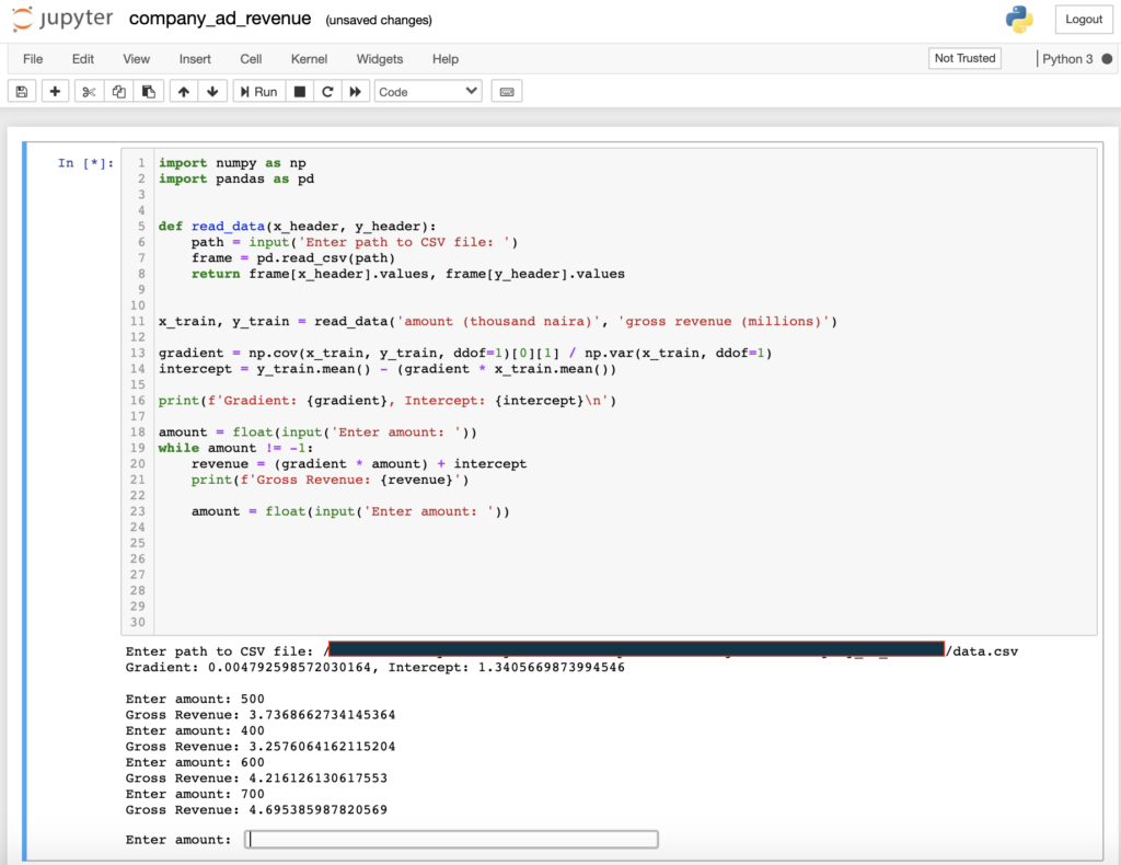
Putting is all together. Here’s what the code looks like:
import numpy as np
import pandas as pd


def read_data(x_header, y_header):
    path = input('Enter path to CSV file: ')
    frame = pd.read_csv(path)
    return frame[x_header].values, frame[y_header].values


x_train, y_train = read_data('amount (thousand naira)',
'gross revenue (millions)')

gradient = np.cov(x_train, y_train, ddof=1)[0][1] / np.var(x_train, ddof=1)
intercept = y_train.mean() - (gradient * x_train.mean())

print(f'Gradient: {gradient}, Intercept: {intercept}\n')

amount = float(input('Enter amount: '))
while amount != -1:
    revenue = (gradient * amount) + intercept
    print(f'Gross Revenue: {revenue}')

    amount = float(input('Enter amount: '))
If you try running this in a Jupyter notebook or from an iPython shell, you should see output like the one below:
Now we can estimate how much the company will make in gross revenue based on the amount spent on advertising.
Wrapping up…
So far, we have been able to dive into some internals of Simple Linear Regression. In a subsequent post, I will re-implement the solution in this post using a library called Scikit-Learn. And then finally, explain some methods for determining the error or suitability of our model.